ChannelTS

A ChannelTS object is a container for a single channel. The data are stored in an xarray.DataArray and indexed by time according to the metadata provided. Here we will make a simple electric channel and look at how to interogate it.

%matplotlib inline
import numpy as np
from mth5.timeseries import ChannelTS
from mt_metadata.timeseries import Electric, Run, Station

Here create some metadata, the keys are the time_period.start and the sample_rate.

ex_metadata = Electric()
ex_metadata.time_period.start = "2020-01-01T00:00:00"
ex_metadata.sample_rate = 8.0
ex_metadata.component = "ex"
ex_metadata.dipole_length = 100.
ex_metadata.units = "millivolts"

Create Station and Run metadata

station_metadata = Station(id="mt001")
run_metadata = Run(id="001")

Create “realistic” data

n_samples = 4096
t = np.arange(n_samples)
data = np.sum([np.cos(2*np.pi*w*t + phi) for w, phi in zip(np.logspace(-3, 3, 20), np.random.rand(20))], axis=0)

ex = ChannelTS(channel_type="electric",
              data=data,
              channel_metadata=ex_metadata,
              run_metadata=run_metadata,
              station_metadata=station_metadata)

ex

Channel Summary:
	Survey:       0
	Station:      mt001
	Run:          001
	Channel Type: Electric
	Component:    ex
	Sample Rate:  8.0
	Start:        2020-01-01T00:00:00+00:00
	End:          2020-01-01T00:08:31.875000+00:00
	N Samples:    4096

Get a slice of the data¶

Here we will provide a start time of the slice and the number of samples that we want the slice to be

ex_slice = ex.get_slice("2020-01-01T00:00:00", n_samples=256)

ex_slice

Channel Summary:
	Survey:       0
	Station:      mt001
	Run:          001
	Channel Type: Electric
	Component:    ex
	Sample Rate:  8.0
	Start:        2020-01-01T00:00:00+00:00
	End:          2020-01-01T00:00:31.875000+00:00
	N Samples:    256

Plot the data¶

This is a work in progress, but this can be done through the xarray container.

ex_slice.plot()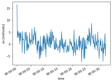

Convert to an `xarray`¶

We can convert the ChannelTS object to an xarray.DataArray which could be easier to use.

ex_xarray = ex.to_xarray()

ex_xarray

ex.plot()
ex_xarray.plot()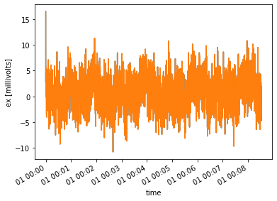

Convert to an `Obspy.Trace` object¶

The ChannelTS object can be converted to an obspy.Trace object. This can be useful when dealing with data received from a mainly seismic archive like IRIS. This can also be useful for using some tools provided by Obspy.

Note there is a loss of information when doing this because an obspy.Trace is based on miniSEED data formats which has minimal metadata.

ex.station_metadata.fdsn.id = "mt001"
ex_trace = ex.to_obspy_trace()

ex_trace

.mt001..MQN | 2020-01-01T00:00:00.000000Z - 2020-01-01T00:08:31.875000Z | 8.0 Hz, 4096 samples

Convert from an `Obspy.Trace` object¶

We can reverse that and convert an obspy.Trace into a ChannelTS. Again useful when dealing with seismic dominated archives.

ex_from_trace = ChannelTS()
ex_from_trace.from_obspy_trace(ex_trace)

ex_from_trace

Channel Summary:
	Survey:       0
	Station:      mt001
	Run:          sr8_001
	Channel Type: Electric
	Component:    ex
	Sample Rate:  8.0
	Start:        2020-01-01T00:00:00+00:00
	End:          2020-01-01T00:08:31.875000+00:00
	N Samples:    4096

ex

Channel Summary:
	Survey:       0
	Station:      mt001
	Run:          001
	Channel Type: Electric
	Component:    ex
	Sample Rate:  8.0
	Start:        2020-01-01T00:00:00+00:00
	End:          2020-01-01T00:08:31.875000+00:00
	N Samples:    4096

On comparison you can see the loss of metadata information.

Calibrate¶

Removing the instrument response to calibrate the data is an important step in processing the data. A convenience function ChannelTS.remove_instrument_response is supplied just for this.
Currently, it will calibrate the whole time series at once and therefore may be slow for large data sets.

See Also: `Make Data From IRIS` examples for working examples.

help(ex.remove_instrument_response)

Help on method remove_instrument_response in module mth5.timeseries.channel_ts:

remove_instrument_response(**kwargs) method of mth5.timeseries.channel_ts.ChannelTS instance
    Remove instrument response from the given channel response filter
    
    The order of operations is important (if applied):
    
        1) detrend
        2) zero mean
        3) zero pad
        4) time window
        5) frequency window
        6) remove response
        7) undo time window
        8) bandpass
    
    **kwargs**
    
    :param plot: to plot the calibration process [ False | True ]
    :type plot: boolean, default True
    :param detrend: Remove linar trend of the time series
    :type detrend: boolean, default True
    :param zero_mean: Remove the mean of the time series
    :type zero_mean: boolean, default True
    :param zero_pad: pad the time series to the next power of 2 for efficiency
    :type zero_pad: boolean, default True
    :param t_window: Time domain windown name see `scipy.signal.windows` for options
    :type t_window: string, default None
    :param t_window_params: Time domain window parameters, parameters can be
    found in `scipy.signal.windows`
    :type t_window_params: dictionary
    :param f_window: Frequency domain windown name see `scipy.signal.windows` for options
    :type f_window: string, defualt None
    :param f_window_params: Frequency window parameters, parameters can be
    found in `scipy.signal.windows`
    :type f_window_params: dictionary
    :param bandpass: bandpass freequency and order {"low":, "high":, "order":,}
    :type bandpass: dictionary

XArray Accessor for Decimate and Filtering¶

A common practice when working with time series would be decimating or downsampling the data. xarray has some builtins for resampling, however these do not apply a filter prior to downsampling and has alias issues. We have added some utilities for decimation and filtering following the package xr-scipy. When MTH5 is initiated a sps_filters accessor to xarray.DataArray and xarray.Dataset which includes some filtering methods as well as decimation and resampling. Therefore for access to these methods use DataArray.sps_filters.decimate or Dataset.sps_filters.decimate.

Methods include

Name	Function
`lowpass`	low pass filter the data
`highpass`	high pass filter the data
`bandpass`	band pass filter the data
`bandstop`	filter out frequencies using a band stop (notch filter)
`decimate`	simulates `scipy.signal.decimate` method by filtering data first then decimating. Can be inaccurate around the edges of the time series because it assumes periodic signal.
`resample_poly`	uses `scipy.signal.resample_poly` method for down sampling, more accurate and usually faster for real signals (default for resampling)
`detrend`	uses `scipy.signal.detrend` with keyword `type` to remove trends in the data

Note: In future versions of MTH5 filters will be added to ChannelTS.

Compare Downsampling methods¶

`Decimate`¶

Here we will decimate to a new sample rate of 1 sample per second.

decimated_ex = ex.decimate(1)

ex.plot()
decimated_ex.plot()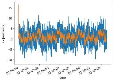

`resample_poly`¶

resample_poly is more accurate for real signals because there is no innate assumption of periodicity. As you can see in the decimate case there are edge effects. Have a look at the scipy documentation for more information. In the plot below, you’ll notice no edge effects and similar numbers as decimate.

Note: Strongly suggest using `ChannelTS.resample_poly` for downsampling data.

resample_poly_ex = ex.resample_poly(1)

ex.plot()
decimated_ex.plot()
resample_poly_ex.plot()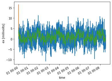

Merge Channels¶

A common step in working with time series would be to combine different segments of collected for the same channel. If the sample rates are the same you can use channel_01 + channel_02. This should also work if the sample rates are not the same, though you should use ChannelTS.merge if the sample rates are not the same. The channels combined must have the same component. There are two builtin methods to combine channels those are + and merge().

added_channel = cnahhel_01 + channel_02
merged_channel = channel_01.merge(channel_02)

Both methods use xarray.combine_by_coords([ch1, rch2], combine_attrs='override'. The combine_by_coords method simply concatenates along similar dimensions and cares nothing of a monotonix dimension variable. Therefore, xarray.DataArray.reindex is used to create a monotonically increasing time series. Any gaps are filled interpolated using a 1-D interpolation. The default method is slinear which is probably the most useful for processing time series. If you want more control over the interpolation method use ChannelTS.merge([ch1, ch2, ...], gap_method=interpolation_method. For more information on interpolation methods see Scipy.interpolate.interp1d. Similarly if you want more control on how the datasets are merged use xarray tools.

Add Channels¶

Adding channels together does 2 at a time so if you are adding multiple channels together channel_01 + channel_02 + channel_03 ... its better to use merge. Also if you want more control on how the channels are merged and how time gaps are interpolated use merge.

ex2 = ex.copy()
ex2.start = "2020-01-01T00:08:45"

added_channel = ex + ex2

added_channel

Channel Summary:
	Survey:       0
	Station:      mt001
	Run:          001
	Channel Type: Electric
	Component:    ex
	Sample Rate:  8.0
	Start:        2020-01-01T00:00:00+00:00
	End:          2020-01-01T00:17:16.875000+00:00
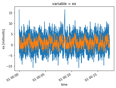
	N Samples:    8296

added_channel.plot()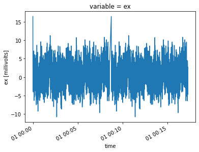

Merge Channels And Resample¶

If channels have different sample rates or you want to combine channels and resample to a lower sample rate, use the keyword argument new_sample_rate.

merged_channel = ex.merge(ex2, new_sample_rate=1)

merged_channel

Channel Summary:
	Survey:       0
	Station:      mt001
	Run:          001
	Channel Type: Electric
	Component:    ex
	Sample Rate:  1.0
	Start:        2020-01-01T00:00:00+00:00
	End:          2020-01-01T00:17:16+00:00
	N Samples:    1037

added_channel.plot()
merged_channel.plot()