RunTS

mth5.timeseries.RunTS is a container to hold multiple synchronous channels of the same sampling rate. The data is contained in an xarray.DataSet which is a collection of ChannelTS.to_xarray() objects.

%matplotlib inline
import numpy as np
from mth5.timeseries import ChannelTS, RunTS
from mt_metadata.timeseries import Electric, Magnetic, Auxiliary, Run, Station

Create a Run¶

We will create a common run that has all 5 channels of an MT measurement (Hx, Hy, Hz, Ex, Ey) plus an auxiliary channel. We will make individual channels first and then add them into a RunTS object.

channel_list = []
common_start = "2020-01-01T00:00:00"
sample_rate = 8.0
n_samples = 4096
t = np.arange(n_samples)
data = np.sum([np.cos(2*np.pi*w*t + phi) for w, phi in zip(np.logspace(-3, 3, 20), np.random.rand(20))], axis=0)

station_metadata = Station(id="mt001")
run_metadata = Run(id="001")

Create `magnetic` channels¶

for component in ["hx", "hy", "hz"]:
    h_metadata = Magnetic(component=component)
    h_metadata.time_period.start = common_start
    h_metadata.sample_rate = sample_rate
    if component in ["hy"]:
        h_metadata.measurement_azimuth = 90
    h_channel = ChannelTS(
        channel_type="magnetic",
        data=data,
        channel_metadata=h_metadata,
        run_metadata=run_metadata,
        station_metadata=station_metadata)
    channel_list.append(h_channel)

Create `electric` channels¶

for component in ["ex", "ey"]:
    e_metadata = Electric(component=component)
    e_metadata.time_period.start = common_start
    e_metadata.sample_rate = sample_rate
    if component in ["ey"]:
        e_metadata.measurement_azimuth = 90
    e_channel = ChannelTS(
        channel_type="electric",
        data=data,
        channel_metadata=e_metadata,
        run_metadata=run_metadata,
        station_metadata=station_metadata)
    channel_list.append(e_channel)

Create `auxiliary` channel¶

aux_metadata = Auxiliary(component="temperature")
aux_metadata.time_period.start = common_start
aux_metadata.sample_rate = sample_rate
aux_channel = ChannelTS(
        channel_type="auxiliary",
        data=np.random.rand(n_samples) * 30,
        channel_metadata=aux_metadata,
        run_metadata=run_metadata,
        station_metadata=station_metadata)
aux_channel.channel_metadata.type = "temperature"
channel_list.append(aux_channel)

Create `RunTS` object¶

Now that we have made individual channels we can make a RunTS object by inputing a list of ChannelTS objects.

Note: This can also be a list of xarray.DataArray objects formated like a channel.

run = RunTS(channel_list)

run

RunTS Summary:
	Survey:      0
	Station:     mt001
	Run:         001
	Start:       2020-01-01T00:00:00+00:00
	End:         2020-01-01T00:08:31.875000+00:00
	Sample Rate: 8.0
	Components:  ['hx', 'hy', 'hz', 'ex', 'ey', 'temperature']

Plot Run¶

Again this is a hack at the moment, we are working on a better visualization, but this works for now.

run.plot()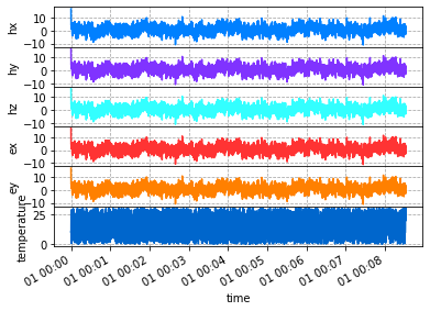

Decimate and Filters¶

A common practice when working with time series would be decimating or downsampling the data. xarray has some builtins for resampling, however these do not apply a filter prior to downsampling and has alias issues. We have added some utilities for decimation and filtering following the package xr-scipy. When MTH5 is initiated a sps_filters accessor to xarray.DataArray and xarray.Dataset which includes some filtering methods as well as decimation and resampling. Therefore for access to these methods use DataArray.sps_filters.decimate or Dataset.sps_filters.decimate.

Methods include

Name	Function
`lowpass`	low pass filter the data
`highpass`	high pass filter the data
`bandpass`	band pass filter the data
`bandstop`	filter out frequencies using a band stop (notch filter)
`decimate`	simulates `scipy.signal.decimate` method by filtering data first then decimating. Can be inaccurate around the edges of the time series because it assumes periodic signal.
`resample_poly`	uses `scipy.signal.resample_poly` method for down sampling, more accurate and usually faster for real signals (default for resampling)
`detrend`	uses `scipy.signal.detrend` with keyword `type` to remove trends in the data

Note: In future versions of MTH5 filters will be added to RunTS.

Compare Downsampling methods¶

`Decimate`¶

Here we will decimate to a new sample rate of 1 sample per second.

decimated_run = run.decimate(1)

2023-09-27T16:30:24.906668-0700 | WARNING | mth5.timeseries.run_ts | validate_metadata | end time of dataset 2020-01-01T00:08:31+00:00 does not match metadata end 2020-01-01T00:08:31.875000+00:00 updating metatdata value to 2020-01-01T00:08:31+00:00

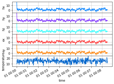
`resample_poly`¶

resample_poly is more accurate for real signals because there is no innate assumption of periodicity. As you can see in the decimate case there are edge effects. Have a look at the scipy documentation for more information. In the plot below, you’ll notice no edge effects and similar numbers as decimate.

Note: Strongly suggest using `RunTS.resample_poly` for downsampling data.

resample_poly_run = run.resample_poly(1)

2023-09-27T16:30:25.076013-0700 | WARNING | mth5.timeseries.run_ts | validate_metadata | end time of dataset 2020-01-01T00:08:31+00:00 does not match metadata end 2020-01-01T00:08:31.875000+00:00 updating metatdata value to 2020-01-01T00:08:31+00:00

decimated_run.plot()
resample_poly_run.plot()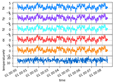

Merge Runs¶

It can be benificial to add runs together to create a longer time series. To combine runs each run must have the same sample rate. There are 2 builtin options for combining runs

added_run = run_01 + run_02
merged_run = run_01.merge(run_02)

Both methods use xarray.combine_by_coords([run1, run2], combine_attrs='override'. The combine_by_coords method simply concatenates along similar dimensions and cares nothing of a monotonix dimension variable. Therefore, xarray.DataSet.reindex is used to create a monotonically increasing time series. Any gaps are filled interpolated using a 1-D interpolation. The default method is slinear which is probably the most useful for processing time series. If you want more control over the interpolation method use RunTS.merge([run1, run2, ...], gap_method=interpolation_method. For more information on interpolation methods see Scipy.interpolate.interp1d. Similarly if you want more control on how the datasets are merged use xarray tools.

Using `+`¶

Using run_01 + run_02 will combine and interpolate onto a new monotonic time index. Any gaps will be interpolated linearly interpolated. If channels are different Nan’s will be placed where channels do not overlap. If you have hz in run_01 but not run_02 then Nan’s will be place in hz for the time period of run_02.

for ch in channel_list:
    ch.start = "2020-01-01T00:08:45"
run_02 = RunTS(channel_list)

added_run = run + run_02

2023-09-27T16:32:27.726365-0700 | WARNING | mth5.timeseries.run_ts | validate_metadata | end time of dataset 2020-01-01T00:17:16.875000+00:00 does not match metadata end 2020-01-01T00:08:31.875000+00:00 updating metatdata value to 2020-01-01T00:17:16.875000+00:00
2023-09-27T16:32:27.726365-0700 | WARNING | mth5.timeseries.run_ts | validate_metadata | sample rate of dataset 8.0 does not match metadata sample rate 1.0 updating metatdata value to 8.0

added_run

RunTS Summary:
	Survey:      0
	Station:     mt001
	Run:         001
	Start:       2020-01-01T00:00:00+00:00
	End:         2020-01-01T00:17:16.875000+00:00
	Sample Rate: 8.0
	Components:  ['hx', 'hy', 'hz', 'ex', 'ey', 'temperature']

Plot combined run¶

Plotting you can see the linear interpolation in the gap of time between the runs. Here it makes a spike because the first point in the time series is a spike.

added_run.plot()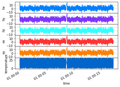

Using Merge and Decimating¶

Using merge is a little more flexible and many runs can be merged together at the same time. Note if you use run_01 + run_02 + run_03 it only combines 2 at a time, which can be inefficient if multiple runs are combined. RunTS.merge provides the option of combining multiple runs and also decimating to lower sample rate with the keyword new_sample_rate.

Runs with different sample rates¶

When using merge not all runs need to have the same sample rate, but you need to set new_sample_rate to the common sample rate for the combined runs. This will decimate the data by first applying an iir filter to remove aliasing and then downsample to the desired sample rate. This mimics scipy.signal.decimate.

Change interpolation method¶

To change how gaps are interpolated change the gap_method parameter. See (scipy.interpolate.interp1d)[https://docs.scipy.org/doc/scipy/reference/generated/scipy.interpolate.interp1d.html]

Options are

‘linear’
‘nearest’
‘nearest-up’
‘zero’
‘slinear’ (default)
‘quadratic’
‘cubic’
‘previous’
‘next’

merged_run = run.merge(run_02, new_sample_rate=1, gap_method="slinear")

2023-09-27T16:32:29.163041-0700 | WARNING | mth5.timeseries.run_ts | validate_metadata | end time of dataset 2020-01-01T00:08:31+00:00 does not match metadata end 2020-01-01T00:08:31.875000+00:00 updating metatdata value to 2020-01-01T00:08:31+00:00
2023-09-27T16:32:29.316779-0700 | WARNING | mth5.timeseries.run_ts | validate_metadata | end time of dataset 2020-01-01T00:17:16+00:00 does not match metadata end 2020-01-01T00:17:16.875000+00:00 updating metatdata value to 2020-01-01T00:17:16+00:00
2023-09-27T16:32:29.499618-0700 | WARNING | mth5.timeseries.run_ts | validate_metadata | end time of dataset 2020-01-01T00:17:16+00:00 does not match metadata end 2020-01-01T00:08:31.875000+00:00 updating metatdata value to 2020-01-01T00:17:16+00:00

merged_run

RunTS Summary:
	Survey:      0
	Station:     mt001
	Run:         001
	Start:       2020-01-01T00:00:00+00:00
	End:         2020-01-01T00:17:16+00:00
	Sample Rate: 1.0
	Components:  ['hx', 'hy', 'hz', 'ex', 'ey', 'temperature']

Plot¶

Plot the merged runs downsampled to 1 second, and the linear interpolation is more obvious.

merged_run.plot()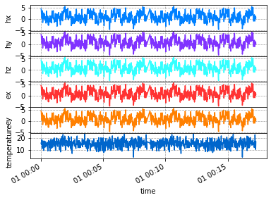

To/From Obspy.Stream¶

When data is downloaded from an FDSN client or data is collected as miniseed Obspy is used to contain the data as a Stream object. Transformation between RunTS and Stream is supported.

To Obspy.Stream¶

stream = run.to_obspy_stream()

stream

6 Trace(s) in Stream:
.mt001..MFN | 2020-01-01T00:00:00.000000Z - 2020-01-01T00:08:31.875000Z | 8.0 Hz, 4096 samples
.mt001..MFE | 2020-01-01T00:00:00.000000Z - 2020-01-01T00:08:31.875000Z | 8.0 Hz, 4096 samples
.mt001..MFZ | 2020-01-01T00:00:00.000000Z - 2020-01-01T00:08:31.875000Z | 8.0 Hz, 4096 samples
.mt001..MQN | 2020-01-01T00:00:00.000000Z - 2020-01-01T00:08:31.875000Z | 8.0 Hz, 4096 samples
.mt001..MQE | 2020-01-01T00:00:00.000000Z - 2020-01-01T00:08:31.875000Z | 8.0 Hz, 4096 samples
.mt001..MKN | 2020-01-01T00:00:00.000000Z - 2020-01-01T00:08:31.875000Z | 8.0 Hz, 4096 samples

From Obspy.Stream¶

new_run = RunTS()
new_run.from_obspy_stream(stream)

new_run

RunTS Summary:
	Survey:      0
	Station:     mt001
	Run:         sr8_001
	Start:       2020-01-01T00:00:00+00:00
	End:         2020-01-01T00:08:31.875000+00:00
	Sample Rate: 8.0
	Components:  ['hx', 'hy', 'hz', 'ex', 'ey', 'temperaturex']